In this paper, we have created and anaysed the Euclid Morphology Challenge, to help the Euclid Consortium in chosing the best software package for the galaxy catalogue production. In this challenge, we asked five galaxy fitting experts to tun their software (DeepLeGATo, Morfometryka, SourceXtractor++, Galapagos-2, and Profit) on a common dataset that we have simulated. They had to predict the Sérsic parameters (flux, half-light radius, Sérsic index and ellipticity) for four different type of images: singe Sérsic, double Sérsic and more realistic simulations (produced by a FVAE, see below). We analysed this complex dataset thanks to three metrics, namely the bias, the dispersion and the outlier fraction. We found a lot of interesting features and comparison, and I describe some of them below.
We first show that most of the codes achieve no major bias and a dispersion below 10% for all single Sérsic parameters. Nevertheless, we identified and anaysed specific behaviours for the dofferent softwares. For example, DeepLeGATo perfoms better for faint objects than bright ones! One could try to use it for faint objets while user ine of the other for bright objects.
In this paper, we simulate realistic galaxies with a Deep Learning model called Flow Variational AutoEncoder (FVAE). The galaxies are learn from real space images, by the Hubble Space Telescope. In addition to the realsitic morphologies learn by the VAE, we also have a good control of the parameters (size, ellipticity and sersic index) thanks to a trained regressive Flow. We used our simulation to forecast the number of interesting galaxies for galaxy science that Euclid will be able to resove. We also created a benchmark to evaluate the relative speed of our model compared to classical simulations.
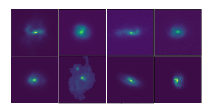
Our model is able to learn complex morphologies. You can see here some examples of spiral arms, rings, clumps and bars. This is done thnaks to a Variational AutoEncoders (VAE). The VAE is amde of two convolutional Neural Networks: an Encoder and Decoder. The Encoder learns the latent distribution of pixels inside a small space, called latent space. The Decoder learns to decode a sample from this representation to recreate the input image. By minimizing the difference between the input image and its reconstruction, we force the representation in the latenstapce to be meaningful. In addition, by regularising the encoded distribution, we can sample this learnt latent space to create new galaxies.
Nevertheless, we don't have any control on the properties of the produced galaxies. This is why we introduce a regressive flow.
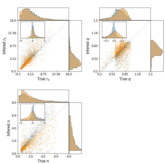
Thanks to the regressive Flow, we learn to map the physical parameter space to the latent space of the trained VAE. In practice, a galaxy with known parameter is encoded by the trained Encoder. Then, the Flow is trained to map this distribution to a Normal Gaussian distribution, conditionned to the physical parameter of the encoded galaxy. Because the transformation is bijective, we can, once trained, transform a sample from a Normal Gaussian distribution to a position in the latent space. If the Flow is well trained, this sample will be decoded to galaxy with the wanted input physical parameters. In the plot on the right, you can see some parameters fitted by a fitting algorithm on our simulated galaxies (orange) and on analytical profiles (blue), versus the true parameter of the simulated galaxy. We see no major departure between blue and orange points, meaning that our Flow is working. The small difference between the two can also be due to the fact that our complexe galaxies are harder to fit by the fitting algorithm.
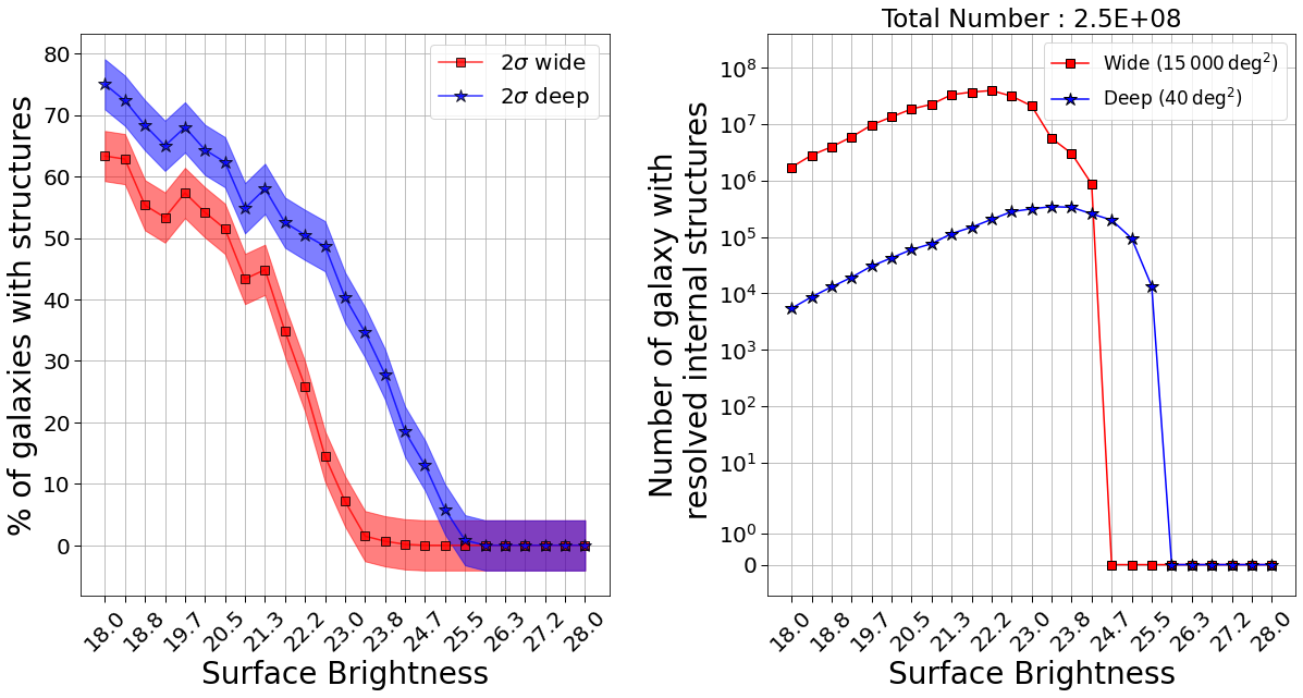
We used our simulation to forecast the number of interesting galaxies for galaxy science that Euclid will be able to resolve. By interesting, we mean galaxies with resolvable structures, irregularities. In the left plot of the figure, we show the percentage of those galaxies regarding the surface brightness of the galaxies. In red for the wide field of Euclid and in blue for the Deep Field. We show that above ~22.5, the wide field will be able to resolve barely no interesting galaxies, and around two magnitude higher for the Deep Field. On the plot on the right, we show the total number of interesting galaxies regarding the surface brightness. Even if the percentage decrease with surface brightness, because the total number of galaxies in the sky is larger at high SB, the total number of interesting galaxies increase at the beginning. In total, we estimate the number of those galaxies to be around 250 millions.
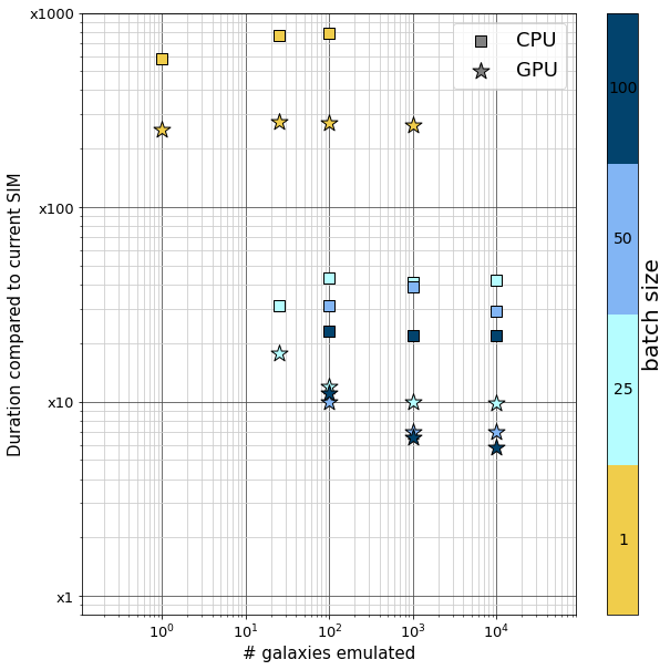
We analysed carefully the running time of our simulations. We compare the time to produce the galaxies to the time made by the simple analytical profiles used in Euclid, which are known to be very fast but very limited regarding the morphology. The plot on the right presents the number of time our model is slower than the analytical simulations, regarding the number of galaxy simulated. It shows three interesting behaviour: our model is always mnore than 5 times faster when using GPUs. It is optimized when producing more galaxies in the same time (batch size, which is the natural behaviour of the model). And our model get faster when the number of simulated galaxies increase and using GPUs compared to the analytical simulation.
In this on-going work published (and refereed) for the Conference on Neural Information Processing Systems (NeurIPS), we explore the use of the probabilistic version of the U-Net (PUnet), recently proposed by Kohl et al. (2018), and adapt it to automate the segmentation of galaxies for large photometric surveys. We focus especially on the probabilistic segmentation of overlapping galaxies, also known as blending. We show that, even when training with a single ground truth per input sample, the model manages to properly capture a pixel-wise uncertainty on the segmentation map. Such uncertainty can then be propagated further down the analysis of the galaxy properties
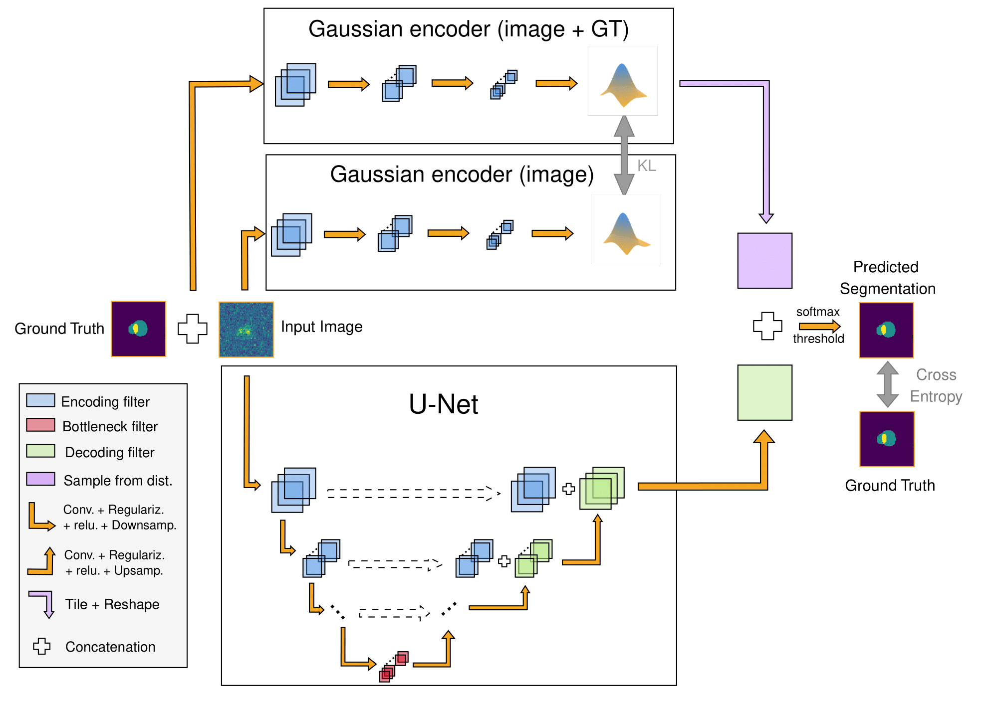
The architecture of the PUnet is made of two parts. On the one hand, there is a classical U-Net (Ronneberger et al., 2015) architecture, whose goal is to create realistic segmentation maps from the input galaxy images. This constitutes the deterministic part of the model. On the other hand, we have an encoder that compresses the images into a Gaussian latent space. This latent space is sampled and concatenated to the output of the U-Net before a final convolution layer to produce the segmentation map. During training, the latent space is regularised using a second encoder that takes as input the ground truth segmentation in addition to the input image. At inference time, that second encoder is removed and the samples are taken only from the latent space of the first encoder. That sampling allows one to have multiple realisations of the segmentation and hence an estimate of the uncertainty at the pixel level.
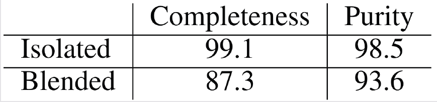
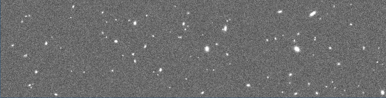
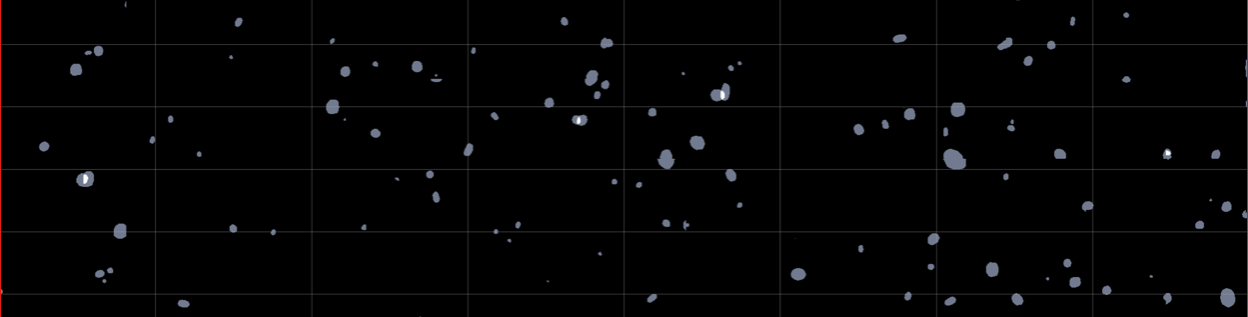
We reconstruct large fields of galaxies by running our model on smaller stamps. Our model achieves very promising results even if our dataset is complex: first, the three classes are strongly imbalanced. ~96% of the pixels belong to the background, ~3% to isolated galaxy, and 1% corresponds to the overlapping regions we would like to focus on. Second, there is a significant fraction of images with no galaxies on them, which we call background stamps. The model could easily fall in a mode where it predicts only background. Finally, because we arbitrarily cut our entire fields into stamps following a fixed grid, a significant amount of galaxies can be cut in the border of the stamps.
INPUT AND TRUE SEGMENTATION
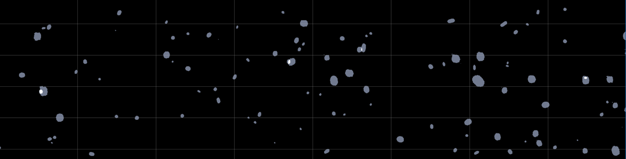
PREDICTION
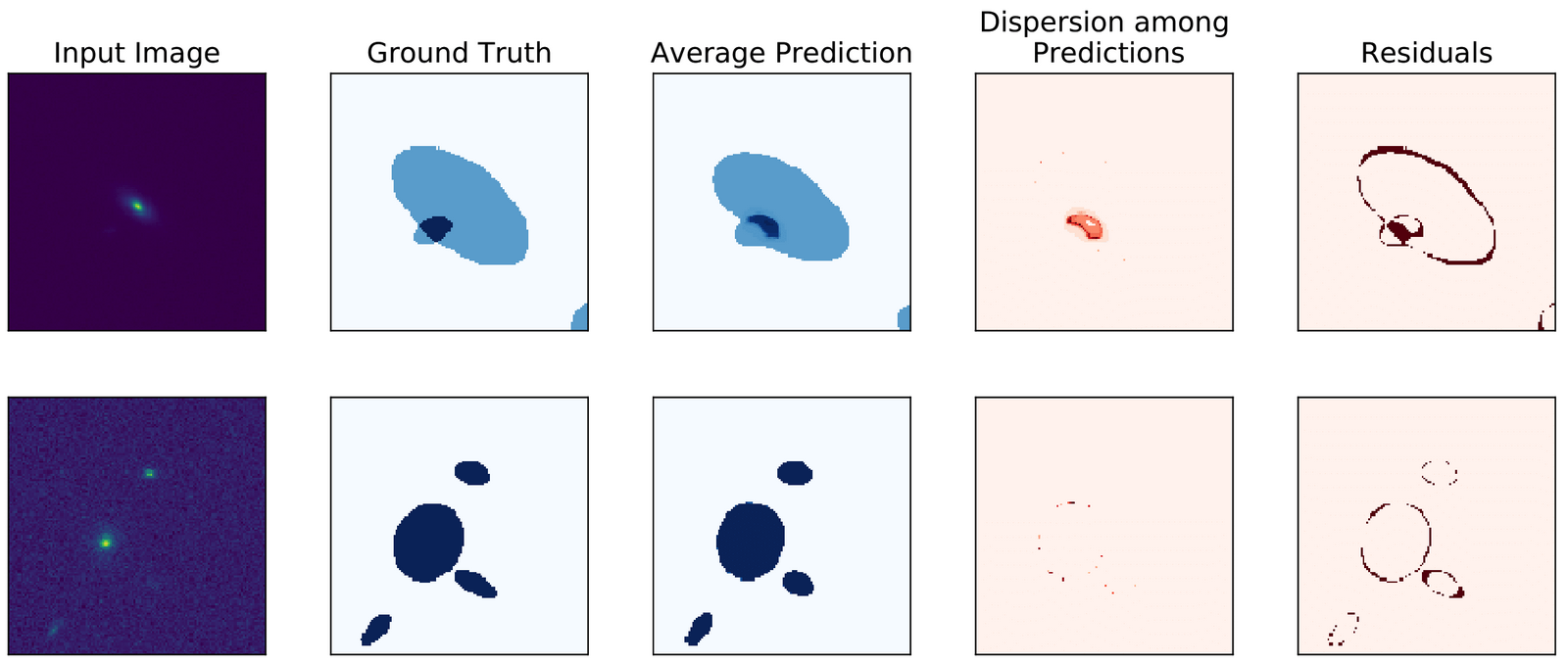
By sampling multiple times the encoded distribution, we can have different realisations of the segmentation for the same image. By taking the mean of those predictions, we have a probabilistic map. By looking at the standard deviation of each pixel with regards to the realisations, we can have a pixel-wise uncertainty. We show here three interesting behaviours. On the first line of the left figure, we can see that even if the model identifies correctly the difficult scene, it is uncertain on the blend region (high variance). On the second line, we can also see that the variance increases on the edges of the galaxies, where the flux is low.
created with
Website Builder Software .